How to Test a Pressure Transmitter Sample: 10 Bench Tests

You have three samples on the bench from two suppliers. Both datasheets say: ±0.25 % FS, IP67, 316L, 4–20 mA. One quote is 40 % lower than the other. The purchase order is for 2,000 pieces, and nobody in the room can say which sample is actually the better transmitter.

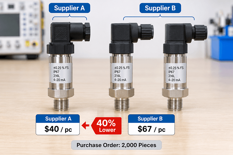
This is how we would want a buyer to test a pressure transmitter sample from us, or from anyone else. The plan uses equipment you can buy for less than one rejected batch costs, takes two working days (three if you run the 72-hour drift test), and ends with a one-page record you can attach to the PO as acceptance criteria.

It is written for the sourcing engineer or buyer and the QA technician they hand the samples to. It assumes you know what a 4–20 mA loop is; if not, start with how a 4–20 mA pressure transmitter works and come back.

The test methods themselves are not new. IEC 60770-1 and IEC 61298-2 define how to test a pressure transmitter under reference conditions. What is missing in most purchasing departments is a short version with numbers in it.

Test a Pressure Transmitter on The Bench

 

Item	Minimum requirement	Why it matters
Pressure source	Hand pump (pneumatic to 40 bar, hydraulic above) or a pressure calibrator	Must reach the proof pressure of the sample, not just full scale
Reference gauge	Digital, at least 4× more accurate than the sample’s spec	A 0.25 % FS sample needs a ≤ 0.06 % reference; a 0.1 % sample needs ≤ 0.025 %
DC power supply	Adjustable 9–32 V, current-limited	Test 6 needs the ends of the supply range, not just 24 V
Current measurement	mA meter with 0.001 mA resolution, or a 250 Ω 0.01 % resistor plus a 5½-digit multimeter	0.01 mA is already 0.06 % of the 16 mA span; coarser meters cannot judge a 0.25 % class unit
Load resistors	250 Ω, 500 Ω, and the maximum from the datasheet	Test 6
Insulation tester	500 V DC	Test 7
Temperature chamber	Or, at minimum, a lab oven to 70 °C and a refrigerator to 0 °C	Test 5 — the test cheap sensors fail most often
Thread gauge, torque wrench	For the process connection on the datasheet	Test 10
Spreadsheet	One row per test point	The record is the deliverable

If you only buy one thing, buy the reference gauge. Everything else can be borrowed; you cannot test a pressure transmitter against a reference that is no better than the transmitter itself, and a poor reference makes every other result meaningless. Our own outgoing calibration uses test Instruments as following:

• Power Supply: (Stabilized Voltage and Current) WM MPS-3503-3;
• Pressure Meter: PACE5000;
• Digital Multimeter : 34401A;
• Insulation ResistaneTester:TH2683

We recommend buyers ask every supplier the same question.

How many samples, and what happens to each

To test a pressure transmitter sample properly, ask for three pieces per model.

1. Serial numbers go into the spreadsheet before anything is powered up.
2. Sample 1 goes through everything including the destructive end of Test 4 and the immersion in Test 10.
3. Samples 2 and 3 run Tests 1–3, 5–7 and 9, and are then stored as golden samples: when the production batch arrives, you compare incoming pieces against them instead of against the datasheet.

One good sample tells you they have a good technician.

Two samples that agree with each other and with the datasheet tell you the supplier has a process.

Test 1 — Paperwork and nameplate (15 minutes)

Check the nameplate against the PO line by line: range, output, supply voltage, process connection, electrical connector, IP rating, hazardous-area marking if ordered, serial number. Then check the calibration certificate: it must name the reference instrument and its calibration date, list the measured points (not just “PASS”), and carry the same serial number as the unit in your hand.

A certificate with no reference instrument on it is a printout, not a certificate. A sample that arrives without a serial number is a sample from a supplier who cannot trace a field failure back to a production lot. Both are reasons to stop before Test 2.

Test 2 — Zero and full scale at room temperature

Connect the sample to the 24 V supply through the mA meter, let it warm up for 15 minutes, apply 0 and 100 % of range from the reference, and read the output.

The ideal output at any pressure is

I_(ideal) = 4 mA + 16 mA × (P – P_(LRV))/(P_(URV) – P_(LRV))

and the error expressed in percent of full scale is

e_(%FS) = (I_(measured) – I_(ideal))/(16 mA) × 100

For a voltage-output unit, replace 4 mA and 16 mA with the zero and span of the output (for 0.5–4.5 V: 0.5 V and 4 V).

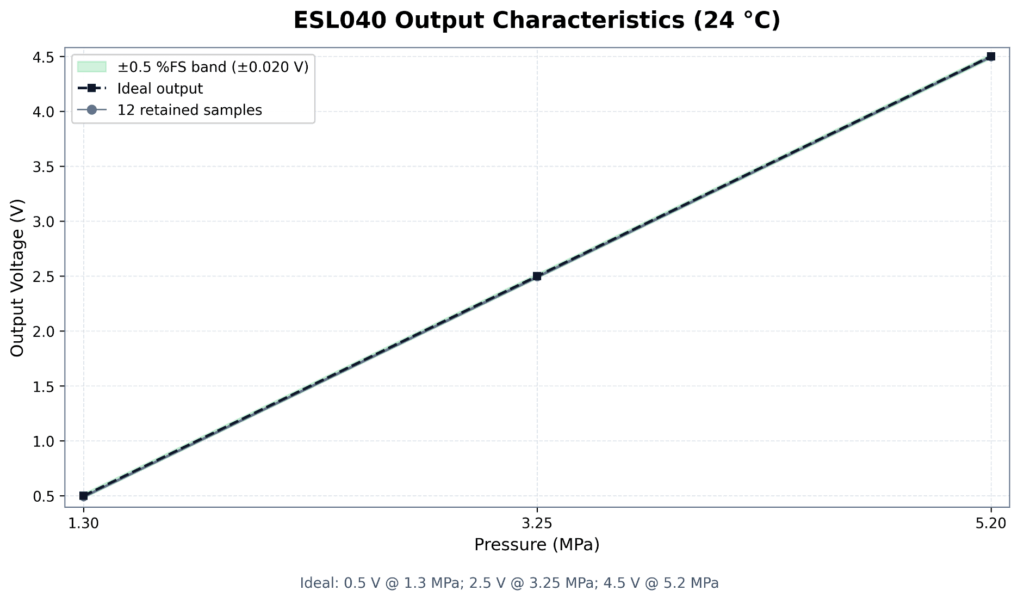
Acceptance. If the datasheet gives separate zero and span setting tolerances, use them. If it only gives an accuracy figure, zero and span must each sit inside it: ±0.04 mA for a 0.25 % class, ±0.08 mA for 0.5 %, ±0.016 mA for 0.1 %. A unit that is already at the edge of its accuracy budget at 25 °C and zero pressure has no margin left for temperature.

 

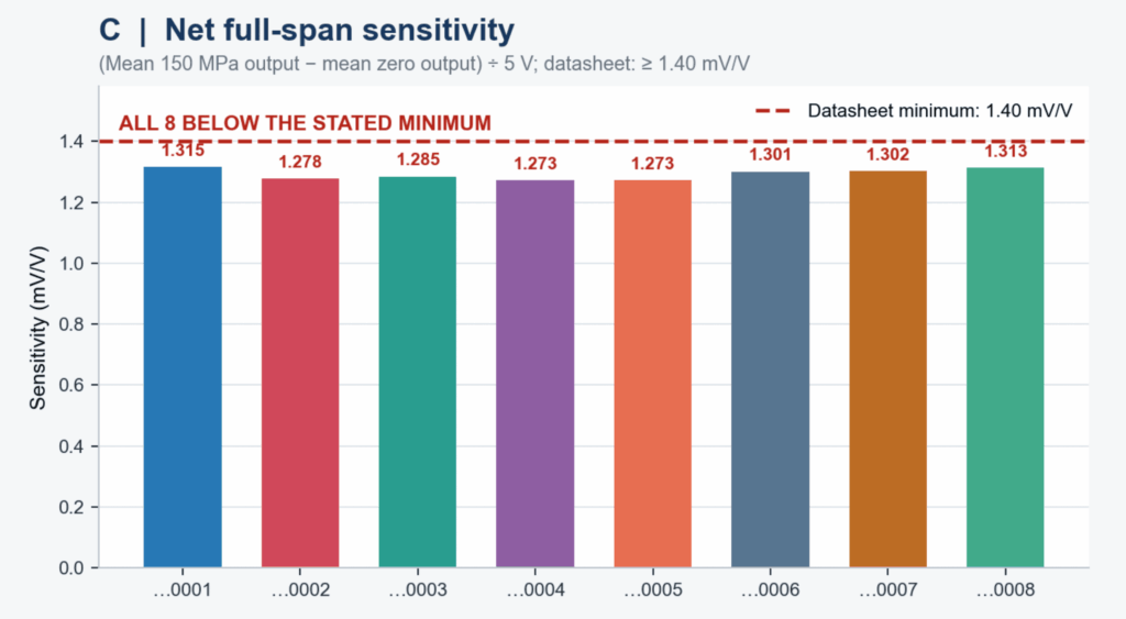
What this looks like on a real record: three of our ESS315-150M thin-film sensor cores (0–150 MPa, millivolt output, 5 V DC supply, S/N 2609270001–0003, tested 2026-10-26) read −0.099 mV, +0.160 mV and −0.014 mV at zero pressure against a datasheet zero tolerance of ≤ ±2 mV. The record is for a sensor core rather than a finished transmitter, so the output column is in mV instead of mA, but the structure is exactly what you want from any supplier: serial number, supply voltage, date, tester, and a measured value next to each specification line rather than the word “PASS”.

Test 3 — Five/Six-point traverse: Linearity, Hysteresis, Repeatability

Apply 0, 25, 50, 75, 100 % of range going up, then 75, 50, 25, 0 % coming down, pausing 30 seconds at each point before reading. Repeat the whole cycle three times. From this one table you read three specifications that most datasheets fold into a single accuracy number:

• Non-linearity is the largest deviation of the upward readings from the straight line, calculated the way the datasheet says (terminal-based or best-fit; they give different numbers, and the datasheet should state which). Background: pressure sensor non-linearity.
• Hysteresis is the largest difference between the upward and downward reading at the same pressure within one cycle. Background: pressure sensor hysteresis.
• Repeatability is the largest spread between the three cycles at the same point and direction. Background: pressure sensor repeatability.

Acceptance. Every reading, up and down, inside the accuracy figure. If hysteresis and repeatability are not broken out on the datasheet, expect each to be under half the accuracy figure. A piezoresistive silicon unit whose hysteresis alone consumes the whole accuracy budget is usually a sign of a stressed die mount or an oil-fill problem, and it will get worse with temperature cycling, not better.

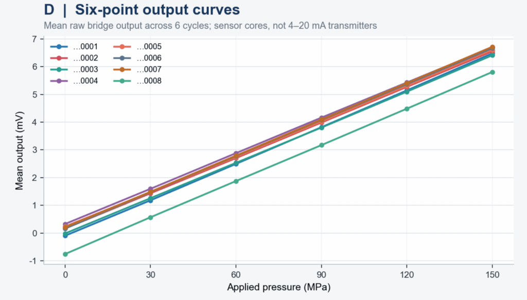
On the three ESS315-150M records mentioned above, each unit was traversed 0–30–60–90–120–150 MPa three times up and three times down, and hysteresis came out at 0.09 %, 0.12 % and 0.09 % FS against a datasheet limit of < 0.15 % FS. The point is not the figure itself; it is that the record lets you see three cycles in both directions per unit, which is the only way to tell hysteresis from repeatability from a single bad reading.

Plot the three cycles. A good transmitter produces three lines you cannot tell apart. A bad one shows you its problem faster than any number does.

Test 4 — Overpressure and recovery

Use Sample 1 only. Apply the proof pressure from the datasheet (commonly 1.5× to 2× full scale for industrial transmitters; some OEM sensors specify more) for five minutes, release, wait ten minutes, and repeat Test 2. Use a liquid medium for anything above 40 bar; compressed gas at proof pressure is an injury waiting to happen.

Then, if you want to know what the sensor is really made of, take Sample 1 up in steps toward the stated burst pressure behind a guard and note where the output stops responding. You will not get this sample back, which is why you asked for three.

Acceptance. Zero shift after proof pressure within the datasheet value, or within the accuracy figure if none is given. Output must return to normal with no permanent offset. The difference between proof and burst, and what each one means for your process, is covered in overpressure, proof pressure and burst pressure.

Test 5 — Temperature: zero and span shift at both ends of the compensated range

Of the ten ways to test a pressure transmitter in this plan, this is the one that separates price tiers, and it is the one buyers skip because it needs a chamber. If you do not have one, a lab oven at 60–70 °C and a refrigerator at 0–5 °C will expose the worst offenders.

Place the sample in the chamber with the pressure port connected by hose to the reference outside (or, in the oven-and-fridge version, test at zero pressure only). Soak for 30 minutes at the low end of the compensated temperature range on the datasheet, read zero and span, then do the same at the high end, then return to 25 °C and read again.

Acceptance. The datasheet gives the limit in one of two forms: a temperature error band such as ±1 % FS over −10 to +70 °C, or a coefficient such as ±0.02 % FS/°C each for zero and span. Convert whichever is given into mA at your test temperatures and compare. A sensing element without active temperature compensation typically shows a zero shift of 2–5 % FS at 70 °C; a compensated one stays inside its band. The physics behind this is in temperature effects on pressure sensors and how temperature causes pressure measurement errors.

The sample should also come back to its 25 °C readings after the cycle. One that does not has a temperature hysteresis problem, which no amount of field calibration will fix.

To show what the datasheet-to-bench comparison looks like in practice: our ESS315 thin-film sensor for drilling and downhole service is specified for a −55 to +175 °C working range with a zero temperature coefficient of ≤ ±0.015 % FS/°C and a sensitivity coefficient of ≤ 0.015 % FS/°C. The outgoing record for each unit includes the zero reading at 20 °C and again after a soak at 50 °C. On the three units above, the zero moved by 0.015 mV over that 30 °C step, which is 0.008 % FS/°C, about half the datasheet allowance. That is the comparison a buyer should be able to make from the paperwork before a unit is ever powered up on their own bench, and it is the first thing to ask for if the supplier’s record stops at room temperature.

Test 6 — Supply voltage and loop load

Run Test 2 at the minimum and maximum supply voltage on the datasheet (typically 9 or 10 V and 30 or 32 V). Then calculate the largest load resistance the loop can drive at your real supply voltage:

R_(L,max) = (U_(supply) – U_(min))/(22 mA)

Datasheets often divide by 20 mA; dividing by 22 mA leaves margin for the fault current of at least 21 mA that NAMUR NE 43 transmitters output when they detect a sensor failure. With a 24 V supply and a 10 V minimum, that is 636 Ω. Put that resistance in the loop at the minimum supply voltage and confirm the output still reaches 20 mA at full scale.

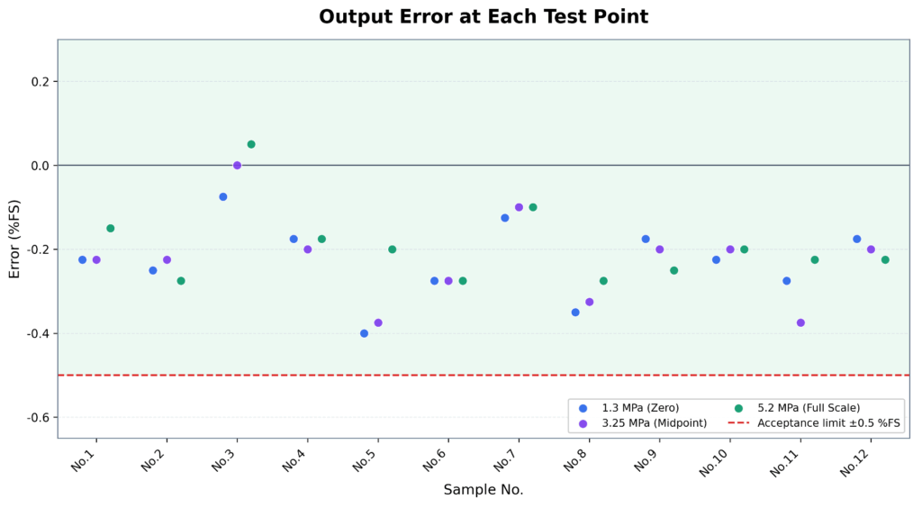
Acceptance. Output change across the supply range within the datasheet figure, typically ≤ 0.01 % FS per volt, so ≤ 0.2 % FS across a 20 V swing. Full 20 mA reached at maximum load and minimum supply. A transmitter that cannot do this will read low at full scale in the field whenever the cable is long or a display is added to the loop. Wiring for 2-, 3- and 4-wire units is in pressure sensor electrical connection; the voltage-output case is in voltage output pressure sensors.

Test 7 — Insulation, reverse polarity, short circuit

Three electrical checks, ten minutes total:

1. Insulation resistance between the housing and all signal pins at 500 V DC. Acceptance: at or above the datasheet value, usually ≥ 100 MΩ. Repeat this after Test 10.
2. Reverse the supply polarity for one minute, restore it, and repeat Test 2. Acceptance: no change in readings. A unit without reverse-polarity protection is a unit that will be destroyed by the first wiring mistake on site.
3. For voltage-output units, short the output to ground for one minute with power applied, then repeat Test 2. Acceptance: no change.

Test 8 — Response time (only if your application needs it)

Skip this for level, static pressure and most process monitoring. Run it for hydraulic systems, pump protection, combustion, test benches and anything with a control loop faster than a few hertz.

Put a fast solenoid valve between a charged reservoir and the sample, put the 250 Ω resistor in the loop and an oscilloscope across it (4–20 mA becomes 1–5 V), open the valve, and measure the time from 10 % to 90 % of the step.

Acceptance. Within the datasheet figure. Amplified piezoresistive OEM sensors are typically in the 1–10 ms range; smart process transmitters with digital filtering are often 100 ms or more, and the damping setting matters more than the sensor. What the number means and how it is specified is in pressure sensor response time. If a supplier’s datasheet gives no response time at all, ask for it before you order; it is one of the first things to be quietly omitted on a low-cost unit.

Test 9 — 72-hour powered drift

Leave Samples 2 and 3 powered at a constant pressure (zero is fine) in a room with stable temperature, and log the output every hour. Any data logger will do; so will a multimeter and a patient technician reading it three times a day.

Acceptance. Total drift ≤ 0.1 % FS over 72 hours, with no steps. Early-life drift is the best cheap predictor you have of the long-term stability figure on the datasheet, which you cannot test in two days. A unit that creeps 0.3 % FS in three days will not meet a ±0.1 % per year stability claim. The mechanisms are explained in pressure sensor drift and long-term stability; a supplier who ages or burns in sensors before calibration will show you a flat line here, and that is worth asking about directly.

A supplier’s outgoing record will normally contain a shorter version of this test. Ours logs the zero at 15, 60, 120, 180 and 240 minutes after power-up at 20 °C; on the three ESS315-150M units the total movement over four hours was 0.002 mV, roughly 0.03 % FS. Four hours is not 72, and we would not expect a buyer to accept it as a substitute. What it tells you is whether the supplier looks at the zero after warm-up at all, and it gives you the starting point your own 72-hour log should match.

Test 10 — Mechanical and ingress

Gauge the thread. Torque the connection to the datasheet value with the supplied sealing and check for leaks at full scale with leak-detection fluid. Inspect the welds, the cable gland or connector seating, and the marking. Then, with Sample 1, verify the IP rating the way the rating defines it: IP65 is a water jet, IP67 is immersion at 1 m for 30 minutes, IP68 is whatever depth and duration the datasheet states. Dry the unit, and repeat the insulation test from Test 7.

Acceptance. No leak at the process connection; insulation resistance unchanged after immersion; no moisture behind the connector or inside the housing. What the IP digits actually promise is in ingress protection ratings explained, and the wetted-material questions that go with this test are in materials of pressure sensors.

 

Reading The Results: What a Failure Tells You

 

What you saw	What is usually behind it	What it means for a 2,000-piece order
Zero and span fine at 25 °C, zero shifts 2 % FS or more at 70 °C	No active temperature compensation, or compensation done at one temperature only	Every outdoor and engine-bay installation will read wrong; field complaints arrive in the first summer
Hysteresis uses up the whole accuracy budget	Stressed die mount, poor oil fill, or a ceramic cell bonded under strain	Gets worse with pressure cycling; expect drift returns within a year
Three cycles in Test 3 do not overlap	Noisy amplifier or unstable reference in the electronics	Will show as unexplained fluctuation on the PLC; impossible to calibrate out
Output cannot reach 20 mA at 636 Ω	Output stage designed for a 250 Ω test load only	Reads low at full scale on any long cable or with a loop display
Insulation below 100 MΩ when new	Potting or sealing defect	Moisture ingress and corrosion within months
72-hour drift above 0.1 % FS	No aging or burn-in before calibration	The calibration certificate describes the unit on the day it was made, not the unit you will install
Certificate without reference instrument or serial number	No traceable calibration process	You cannot audit a batch, and the supplier cannot trace a complaint

None of these appear on a datasheet. All of them appear within two days when you test a pressure transmitter sample on a bench.

 

Writing It into The Purchase Order

 

Once the samples have passed, the test record becomes the acceptance criterion for the batch. Three clauses are enough:

1. Reference. “Supplied units shall conform to the performance of approved samples S/N [numbers], test record dated [date], attached.”
2. Batch evidence. “Supplier shall provide serial-level calibration data for 100 % of units, including the reference instrument identification and the five-point readings, in electronic form before shipment.”
3. Incoming inspection. “Buyer may select [n] units per lot at random and repeat Tests 2, 3 and 7 of the attached record; a failure of any unit entitles Buyer to reject the lot.”

Ask the supplier four things while you are at it:

1. Which reference standard their calibration is traceable to and when it was last calibrated;
2. Whether sensors are aged or burned in before calibration, and for how long;
3. What their process capability is on the accuracy figure (a supplier running at Cpk 1.33 on ±0.25 % will tell you; one running at the edge will change the subject); 
4. Whether they will share the chamber data for the temperature compensation of your specific range.

The answers tell you more than the price does.

A supplier whose samples pass when you test a pressure transmitter this way is not necessarily the cheapest. But the gap between the quotes shrinks quickly once you add the cost of a field failure on a machine that has already shipped, and the supplier who passes is the one whose next batch will look like the samples.

 

Frequently Asked Questions